A French research group has asserted that multiple concave margins are more common in benign lesions and tumors on long bones, and this feature might help assist radiologists in making a diagnosis.
In an article published in Insights into Imaging on 10 November, a team led by Dr. Abdulrazak Kalaaji, of the Department of Musculoskeletal Imaging, CIAL, Lille University Hospital, conducted a retrospective observational study of focal intraosseous lesions of the long bones identified on MRI exams.
 Lesions with at least two concave borders (arrows): a, b osteonecrosis; c, d fibrous dysplasia.Kalaaji et al; Insights Into Imaging
The analysis included 586 lesions from 494 patients; 296 (50.5%) were observed in male patients and 290 (49.5%) in female patients, with a median age of 46 (age range: 14 months to 86 years). Of the patients, 441 (89.3%) had one lesion, 33 (6.7%) had two, and 20 (4%) had between three and seven.
The margins of lesions in the analysis were classified as concave (having at least one focal concavity or a complete concave margin, with a smooth and regular inward-curved contour), not concave, or cortical (when the lesion margin was predominantly in contact with the cortex, which prevented reliable analysis).
The analysis included 15 different types of lesions (75.1% were tumors; 24.9% were nontumoral lesions). The number of concave margins per lesion varied significantly by lesion type (p < 0.001).
 Lesions with concave borders (arrows): (a, b) intraosseous abscess, (c) chondroblastoma, (d) Langerhans cell histiocytosis, and (e, f) metastasis (same patient). In (a) and (c), one concave border follows the shape of the growth plate.Kalaaji et al; Insights Into Imaging
All osteonecrosis lesions, 44.8% of fibrous dysplasia lesions, 20.8% of abscesses, 14.8% of chondroblastomas, 12.5% of Langerhans cell histiocytosis lesions, and 2.9% of metastases showed at least two concave margins. No lesions in the other groups had more than one concave margin.
Nontumoral lesions had more frequent concave margins than tumoral lesions (p < 0.001). Benign lesions (nontumoral lesions and benign tumors) had more frequent concave margins than intermediate and malignant tumors (p < 0.001). After excluding osteonecrosis lesions, this difference remained statistically significant (p = 0.0075).
The second most common bone lesion with concave margins (following osteonecrosis) was fibrous dysplasia. Almost half of the lesions in the analysis had at least two concave margins. After the exclusion of osteonecrosis, the presence of two or more concave margins yielded a positive predictive value (PPV) of 0.76.
This finding has not been previously reported, the authors stated. “The depiction of at least two concave margins in lesions with non-fatty signal intensity might be useful for recognizing fibrous dysplasia and could be considered a reassuring feature.”
Of 34 metastasized lesions, only one had two concave borders. The authors suggest that the reason for this outlier lesion may have been its small size and the “relatively indolent behavior” caused by the underlying neuroendocrine renal primary tumor; however, they caution that the rarity of this would need to be confirmed in future analyses.
Nevertheless, the study findings suggest that the presence of at least two smooth inward-curving margins on MRI is more common in benign lesions; when this feature is present in nonfatty lesions, it could have utility in identifying fibrous dysplasia, they concluded.
Read the full paper here.