New method painlessly measures gadolinium in bone

The routine use of gadolinium-based contrast agents for MRI is under scrutiny due to recent evidence of gadolinium deposition in the bones of healthy individuals. In addition, some individuals who received this contrast have exhibited symptoms associated with gadolinium toxicity. Therefore, there's a pressing need for an in vivo measurement technique that can assess gadolinium deposition in bone.

Currently, gadolinium levels in bone can only be measured through painful invasive techniques. To address this, researchers from Ryerson University and McMaster University are investigating the use of noninvasive x-ray fluorescence (XRF) to detect gadolinium in bone. The team has developed an XRF system that has successfully measured gadolinium in bone phantoms and autopsy bone samples. For in vivo use, however, interpatient variability -- such as the source-to-measurement site distance, bone size, and the depth of overlying tissue -- creates an additional challenge.

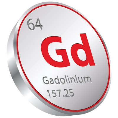
X-ray fluorescence system performing a human tibial measurement to detect gadolinium. Image credit: Paulina Rzeczkowska.

To correct for interpatient variability, the Canadian team is exploring the use of coherent normalization, which involves normalizing the gadolinium K x-ray peak to the coherent peak of the excitation source. In their latest work, they used phantom-based experiments and Monte Carlo simulations to demonstrate the feasibility of this approach (Physiological Measurement, 21 September 2017).

"The XRF system has been successfully used to account for tissue thickness variability in measurements of lead for many years in our research group," explained co-first author Michelle Lord, a doctoral student at McMaster. "Having the same excitation source and geometry as the lead XRF setup, the only difference was that gadolinium was being detected instead of lead. For this reason, we decided to try coherent normalization as our first approach, which ended up working well."

Phantom studies

Lord and colleagues created a tibia phantom using plaster of Paris to represent bone, mixed with 120 µg gadolinium/g plaster. They mounted a Cd-109 excitation source (which emits 88 keV gamma-rays) to the face of a clover-leaf high-purity germanium detector, and placed the phantom 1 mm in front of the source.

Gadolinium K x-ray counts normalized to the Cd-109 coherently scattered gamma-rays for experiments and simulations.

To investigate how the ratio of gadolinium signal to coherent peak signal changed with tissue thickness, the team measured the bone phantom within cylinders of Solid Water, inserted at depths of 3.3, 4.0, 7.5, and 12.2 mm to represent different tissue thicknesses. For each measurement, they calculated the areas of the two gadolinium K peaks (at 42.3 and 43 keV) and the coherent peak (at 88 keV).

Plotting gadolinium K x-ray counts normalized to the 88 keV coherently scattered gamma-rays as a function of tissue thickness resulted in a line with a slope of zero (0.0021 ± 0.0059), for tissue thicknesses from 0 mm to 12.2 mm, suggesting that coherent normalization is valid over the entire thickness range.

MC simulations

In work led by Zaid Keldani at Ryerson, the researchers also used the Monte Carlo N-Particle radiation transport code MCNP6 to model the XRF system, including the detection system, collimator, phantom, and Solid Water. In the simulations, normalizing the gadolinium K x-ray signal to the coherently scattered signal as a function of tissue thickness resulted in a line with a slope of -0.0053 ± 0.0040, again suggesting that the normalization method is effective for tissue thicknesses of up to 12.2 mm.

For tissue thicknesses of 3.3 mm to 7.5 mm, Monte Carlo simulations resulted in an insignificant slope of -0.0043. Because the average tissue thickness over an adult tibia is 4 mm to 5 mm, this shows that coherent normalization is especially useful for average healthy individuals.

The average simulated gadolinium-to-coherent signal ratio was 0.717 ± 0.025, in good agreement with the measured value of 0.749 ± 0.019. The authors concluded that the simulations validated their experimental results and demonstrated that coherent normalization for the XRF system was effective to better than 5% over a large range of tissue thicknesses.

Keldani notes the gadolinium XRF system is still some way from being used in the clinic. "Now that we have validated that coherent normalization works well for individuals with average tissue thicknesses over the tibia, we can use this approach to eliminate interpatient tissue variation when performing human measurements," he said. "We still need to investigate the ability of coherent normalization to correct for interpatient variation in bone size."

The researchers have, however, recently used their XRF system to conduct the first in vivo measurements of gadolinium in bone, in 11 individuals exposed to gadolinium-based contrast agents and 11 controls. "We found a significant difference in gadolinium bone concentration between the two groups," Lord said. "We believe this is just the tip of the iceberg and there is a lot more to unfold regarding gadolinium deposition in the body."

© IOP Publishing Limited. Republished with permission from medicalphysicsweb, a community website covering fundamental research and emerging technologies in medical imaging and radiation therapy.